2022.07.25 - [Studying/Machine Learning] - [머신러닝] CIFAR-10 이미지 분류 - VGG-19 모델
[머신러닝] CIFAR-10 이미지 분류 - VGG-19 모델
2022.07.22 - [Studying/Machine Learning] - [머신러닝] CNN 모델 구현 with Pytorch (CIFAR-10 dataset) [머신러닝] CNN 모델 구현 with Pytorch (CIFAR-10 dataset) 2022.07.21 - [Studying/Machine Learning]..
gm-note.tistory.com
저번 포스트에서 사전학습 모델을 가져와서 학습을 진행했었다.
이번에도 사전학습 모델을 가져와서 style transfer를 해보겠다.
Introduction
먼저 Style Transfer 소개를 하겠다.
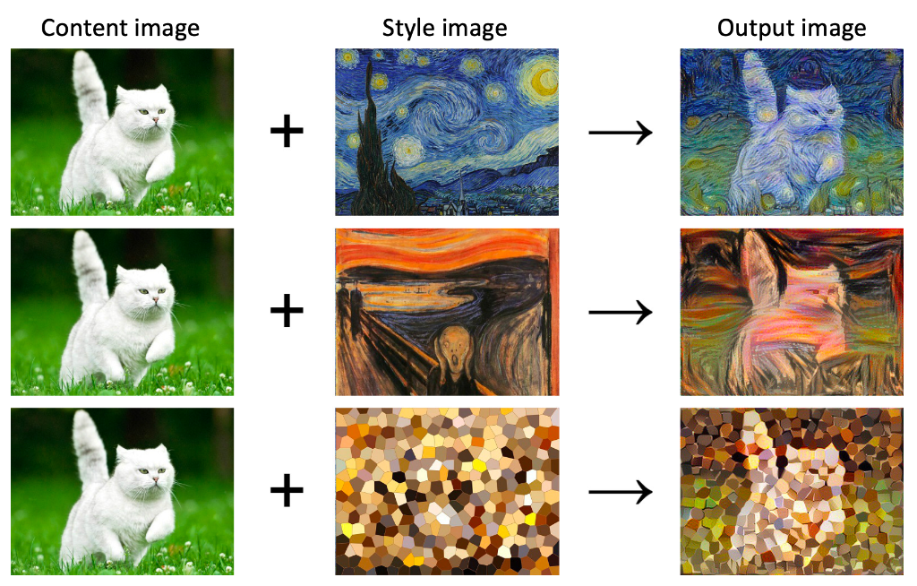
style transfer는 한 이미지에 다른 이미지의 스타일을 적용해서 새로운 이미지를 생성하는 방식이다.
방식은 여러 가지가 있는데 사전 학습된 모델을 가져와서 content 이미지와 style 이미지를 입력으로 넣어서
이미지를 학습하는 tutorial을 해보려고 한다.
Model Structure
모델 구조를 간단하게 보겠다.
상세하게 설명하기엔 원리까지 깊이 들어가야 하지만
이 포스트의 목적은 tutorial이므로 기초적인 프로세스를 설명하겠다.
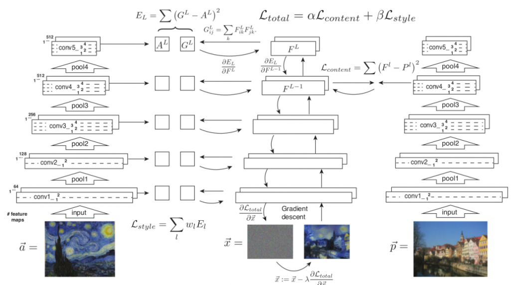
우선 content 이미지인 a, style 이미지인 p, 결과물이 될 x는 노이즈로 초기화하고 시작한다.
그리고 신경망에 각 이미지들을 통과 시킨다. 이때 style 이미지는 Gram matrix를 사용한다.
사용 이유는 쉽게 설명하면 여러 layer의 feature map을 같이 확인하며 style을 추출하기 위함이다.
여기서 a,x에 대해서는 style의 loss를 계산한다.
여기서의 loss 계산은 살짝 변형이 되는데 각 layer에서 loss를 계산한 후
여러 레이어를 동시에 보고 계산해야 하므로 각 layer의 loss에 가중치를 곱해 그 합을 계산한다.
그리고 p,x에 대해서는 각 layer에서 content loss를 계산한다.
그리고 두 loss에 가중치를 각각 곱해서 더한다.
이 가중치에 따라 스타일을 더 많이 따라갈 것인지, 콘텐츠를 더 많이 따라갈 것인지 학습된다.
이 합쳐진 loss를 back propagation해서 이미지 x를 업데이트한다.
Code
우선 필요한 모듈들을 불러온다.
import os
os.environ['CUDA_VISIBLE_DEVICES'] = '0'
import numpy as np
from PIL import Image	#이미지 처리
import matplotlib.pyplot as plt	#그래프
from tqdm.notebook import tqdm
import torch
import torch.nn as nn
import torchvision
from torchvision import models
from torchvision import transforms
학습에 사용될 hyperparameter 값을 넣을 class를 먼저 정의한다.
class AttrDict(dict):
    def __init__(self, *args, **kwargs):
        super(AttrDict, self).__init__(*args, **kwargs)
        self.__dict__ = self
hyperparameter를 세팅해준다.
여기서 기본적인 저장 경로나 에포크, 이미지 크기들도 정의했고,
입력 이미지에 적용할 normalize와 출력 이미지에 적용할 denormalize도 정의한다.
여기서 normalize 값은 사전학습에 사용된 ImageNet 데이터셋 학습에서 얻어낸 값들이다.
config = AttrDict()
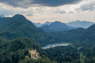
config.content_img = 'data/mountain.jpg'
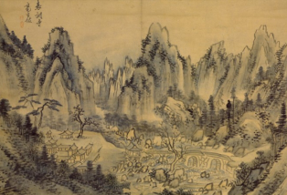
config.style_img = 'data/muk.jpg'
config.save_path = 'save/'
config.n_step = 200
config.log_interval = 50
config.save_interval = 50
config.style_loss_weight = 1
config.learning_rate = 0.1
config.img_size = 512
config.augmentation = transforms.Compose([
transforms.Resize(config.img_size),
transforms.ToTensor(),
transforms.Normalize(mean=(0.485, 0.456, 0.406), std=(0.229, 0.224, 0.225))
])
config.denormalize = lambda x:x*torch.tensor([[[0.229]], [[0.224]], [[0.225]]])+torch.tensor([[[0.485]], [[0.456]], [[0.406]]])
config.device = torch.device('cuda' if torch.cuda.is_available() else 'cpu')이미지는 다음과 같이 산과 동양화 이미지를 사용했다.
style transfer는 재미로 많이 사용하기에 설정도 저장해 놓겠다.
if not os.path.isdir(config.save_path):
    os.makedirs(config.save_path)
이미지를 불러와서 torch tensor로 바꾸는 함수를 정의한다.
def image_preprocess(image_path, transform=None):
    image = Image.open(image_path)

    if transform:
        image = transform(image)

    return image.unsqueeze(0).to(config.device)
그리고 이미지 전처리를 수행한다. target 이미지는 content 이미지로 초기값을 설정하겠다.
content_img = image_preprocess(config.content_img, config.augmentation)
style_img = image_preprocess(config.style_img, config.augmentation)

target_img = content_img.clone().requires_grad_(True)
ImageNet으로 사전 학습된 vgg19 모델의 features를 가져오겠다.
model = models.vgg19(pretrained=True).features
이제 이미지를 vgg19에 통과시켜 5개의 layer에서 feature를 뽑아 리턴하는 모델을 정의한다.
레이어는 랜덤이 아니고 논문에서 사용한 layer 번호이다.
class feature_model(nn.Module):
    def __init__(self):
        super(feature_model, self).__init__()
        self.model = models.vgg19(pretrained=True).features
        self.selected_layer = ['0', '5', '10', '19', '28']

    def forward(self, x_list):
        feature_list = []
        for x in x_list:
            feature_list.append(self._forward(x))
        return feature_list

    def _forward(self, x):
        selected_features = []
        for n, layer in self.model._modules.items():
            x = layer(x)
            if n in self.selected_layer:
                selected_features.append(x)
        return selected_features
optimizer과 loss function을 설정해준다.
model이 아닌 image를 업데이트하는 것이므로 optimizer에 이미지를 넣어준다.
optimizer = torch.optim.Adam([target_img], lr=config.learning_rate)
criterion = nn.MSELoss()
model = feature_model().to(config.device)
model.eval()
Training
for i in tqdm(range(config.n_step)):
    c, s, t = model([content_img, style_img, target_img])

    style_loss = 0
    content_loss = 0
    for content_feature, style_feature, target_feature in zip(c, s, t):
    	#content loss
        content_loss += criterion(target_feature, content_feature)

        #style loss를 구하기 위해 target image와 style image의 gram matrix를 계산한다
        style_feature = style_feature.reshape(style_feature.shape[1], -1)
        target_feature = target_feature.reshape(target_feature.shape[1], -1)
        style_feature = torch.mm(style_feature, style_feature.t())
        target_feature = torch.mm(target_feature, target_feature.t())

        #style loss
        style_loss += criterion(target_feature, style_feature) / (style_feature.shape[0] * style_feature.shape[1])

    #total loss
    loss = content_loss + style_loss * config.style_loss_weight

    optimizer.zero_grad()
    loss.backward()
    optimizer.step()

    if (i+1) % config.log_interval == 0:
        print('Epoch [{}/{}] Content loss: {:.4f} Style loss: {:.4f}'
                   .format(i+1, config.n_step, content_loss.item(), style_loss.item()))

    if (i+1) % config.save_interval == 0:
        save_path = os.path.join(config.save_path,
                                 'content_[{}]_style_[{}]_weight_[{}]_epoch_[{}].png'.format(config.content_img.split('/')[-1],
                                                                                             config.style_img.split('/')[-1],
                                                                                             config.style_loss_weight, i+1))
        save_img = target_img.squeeze(0).data.cpu()
        save_img = config.denormalize(save_img).clamp(0., 1.)
        torchvision.utils.save_image(save_img, save_path)
이미지 생성이 완료되었으니 결과 확인을 위해 시각화를 해주는 함수를 정의해준다.
def draw_images(content_img, style_img, target_img, target_img_name):
    plt.figure(figsize=(20, 60))
    plt.subplot(1, 3, 1)
    plt.title('content image')
    plt.imshow(content_img)

    plt.subplot(1, 3, 2)
    plt.title('style image')
    plt.imshow(style_img)

    plt.subplot(1, 3, 3)
    plt.title(target_img_name)
    plt.imshow(target_img)
    plt.show()
결과를 확인해보겠다.
content_img = Image.open(os.path.join(config.content_img))
style_img = Image.open(os.path.join(config.style_img))

name = 'content_[{}]_style_[{}]'.format(config.content_img.split('/')[-1], config.style_img.split('/')[-1])
for image_path in os.listdir(config.save_path):
    if image_path.startswith(name):
        target_img = Image.open(os.path.join(config.save_path, image_path))
        draw_images(content_img, style_img, target_img, image_path)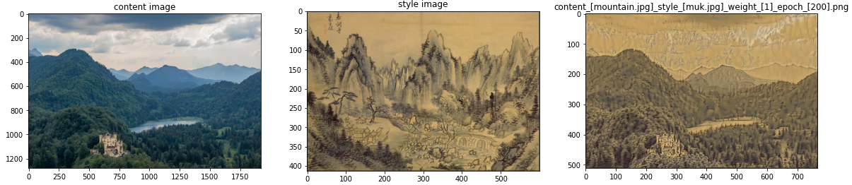
산이 동양화 스타일로 잘 표현된 것을 확인할 수 있다.
References
Leon A. Gatys, Alexander S. Ecker, Matthias Bethge, A Neural Algorithm of Artistic Style(2015), arXiv
이렇게 style transfer를 해봤다.
이 부분이 KAIST에서 머신러닝을 배우며 가장 흥미로웠던 부분이다.
기본적인 지식이 없어도 따라 할 수 있도록 간단하게 만들어져 있어서 한번 해봐도 좋을 것 같다.
둘이 경향이 많이 다른 이미지는 조금 더 큰 모델로 더 많은 epoch를 학습해보면 잘 나오긴 한다.
원하는 대로 나오지 않는다면 style_loss_weight를 바꾸면서 해보면 어느 정도 보완이 될 것 같다.
'Studying > Machine Learning' 카테고리의 다른 글
| [머신러닝] 자연어 처리 파이썬 모듈 (NLP Python module) (4) | 2022.08.03 |
|---|---|
| [머신러닝] 파이썬 정규 표현식 regex (1) | 2022.08.01 |
| [머신러닝] CIFAR-10 이미지 분류 - VGG-19 모델 (5) | 2022.07.25 |
| [머신러닝] Local optimum이란? (0) | 2022.07.25 |
| [머신러닝] CNN 모델 구현 with Pytorch (CIFAR-10 dataset) (2) | 2022.07.22 |


댓글